Leapfrog Probing
- A hash table is a data structure that stores a set of items, each of which maps a specific key to a specific value.
- There are many ways to implement a hash table, but they all have one thing in common: buckets.
- Every hash table maintains an array of buckets somewhere, and each item belongs exactly to one bucket.
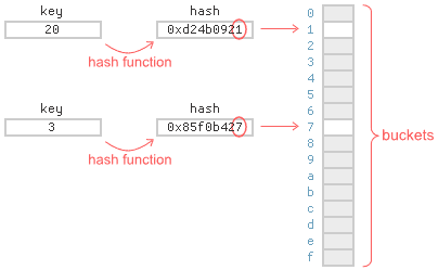
- To determine the bucket for a given item, you typically hash the item's key, then compute its modulus - that is, the remainder when divided by the number of buckets.
- For a hash table of 16 buckets, the modulus is given by the final hexadecimal digit of the hash.
- Inevitably, several items will end up belonging to same bucket.
- For simplicity, lets suppose the hash function is invertible, so that we only need to store hashed keys.
- A well-known strategy is to store the bucket contents in a linked-list:
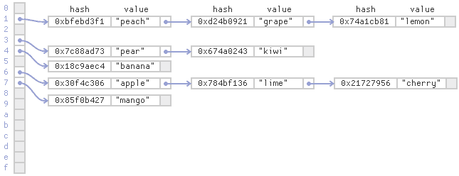
- This strategy is known as separate chaining.
- Separate chaining tends to be relatively slow on modern CPUs, since it requires a lot of pointer lookiups.
- There is other concept called open addressing which stores all the items in the array itself.
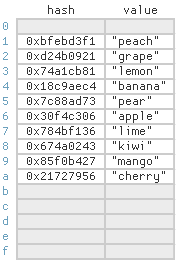
- In oopen addressing, each cell in the array still represents a single bucket, but can actually store an item belonging to any bucket.
- Open addressing is more cache-friendly that separate chaining.
- If an item is not found in its ideal cell, it is often nearby.
- The drawback is that as the array becomes full, you may need to search a lot of cells before finding a particular item, depdending on the probing strategy.
- For example, consider linear probing, the simplest probing strategy.
- Suppose we want to insert the item into the above table, and the has of 13 is
0x95bb7d92. - Ideally we would store this item at index 2, the last hexadecimal digitj of the hash, but that cell is already taken.
- Under linear probing, we find the next free cell by searching linearly, starting at the item's ideal index, and store the item there instead.
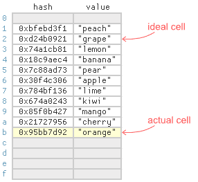
- As you can see, the item ended up quite far from its ideal cell.
- Not great for lookups.
- Everytime someone calls
getwith this key, they'll have to search cells 2 through 11 before finding it. - As the array becomes full, long searches become more and more comon.
- There are alternatives to linear probing, such as quadratic probing.
- There is other strategy called
Leapfrog Probing.
Finding Existing Items
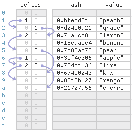
- In Leapfrog Probing, we store two additional delta values for each cell.
- These delta values define an explicit probe chain for each bucket.
-
To find a given key, proceed as follows
- First, hash the key and compute its modulus to get the bucket index. That's the item's ideal cell. Check there first.
- If the item isn't found in that cell, use that cell's first delta value to determine the next cell to check. Just add the delta value to the current array index, making sure to wrap at the end of the array.
- If the item isn't found in that cell, use the second delta value foor all subsequent cells. Stop when the delta is zero.
-
For the strategy to work, there really needs to be two delta values per cell.
-
The first delta value directs us to the desried bucket's probe chain and the second delta value keeps us in the same probe chain.
- For example, suppose we look for the key 40 in the above table, and 40 hashes to
0x674a0243. - The modulus is 3, so we check index 3 first, but index 3 contians an item belonging to a different bucket.
- The first delta valu at index 3 is
2, so we add that to the current index and check index 5. - The item isn't there either, but at least index 5 contains an item belongingg to the desired bucket, since its hash also ends with 3.
- The second delta valu at index 5 is
3, so we add that to the current index and check index 8. - At index 8, the hashed key
0x674a0243is found.
- A single byte is sufficient to store each delta value.
- If the hash table's keys and values are 4 bytes each, and we pack the delta values together, it only takes 25% addition memory to add them.
- If they keys and values are 8 bytes, the additional memory is 12.5%.
Inserting New Items
- Inserting an item into a leapfrog table consists of two phases:
- following the probe chain to see if an item with the same key already exists, then, if not,
- performing a linear search for a free cell.
- The linear search begins at the end of the probe chain.
- Once a free cell is found and reserved, it gets linked to the end of the chain.
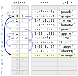
- For example, suppoose we insert the same item , with hash
0x95bb7d92. - The item's bucket index is 2, but index 2 already contains a different key.
- The first delta value at index 2 is zero, which marks the end of the probe chain.
- We proceed to the second phase:
- Performing linear search starting at index 2 to locate the next free cell.
- As before, the item ends up quite far from its ideal cell, but this tieme, we set index 2's first delta value
9, linking the item to its probe chain. - Now subsequent lookups will find the item more quickly.
- Of course, any time we search for a free c ell, the cell must fall withing reach of its designated probe chain.
- In other words, the resulting delta value must fit into a single byte.
- If the detla value does not fit, the the table is overpopulated, and its time to migrate its entire contents to a new table.